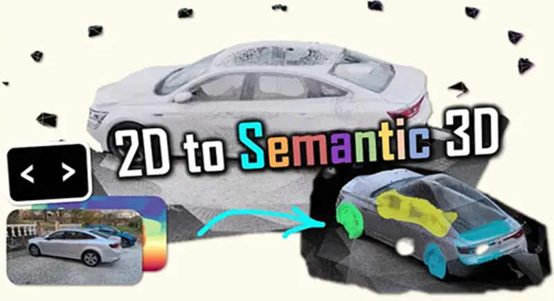
从图像到语义3D高斯散点

如果您曾经尝试在密集的 3D 点云中分割特定对象（例如路牌或汽车轮胎），您一定深有体会。

您旋转视口，眯着眼睛盯着屏幕，试图用套索工具捕捉一团看起来像一团模糊汤的点。

感觉就像戴着拳击手套做显微外科手术一样。

不过，我从未做过显微外科手术，也从未日常佩戴拳击手套，所以我的比喻可能略显局限。

然而，标注二维图像却轻而易举。一个孩子就能在照片中画一个圈圈出汽车。

那么，既然我们可以利用像素，为什么还要与几何形状作斗争呢？

我们将迎来空间人工智能的巨大变革：从被动重建（仅仅捕捉几何形状并祈祷它看起来不错）转向主动语义注入。

我们需要的不仅仅是点，而是意义。

虽然像“Map Anything”这样的工具专注于高级拓扑布局，但Depth Anything V3 (DA3) 更进一步，仅需一台摄像机即可生成密集的度量几何图形。

它使我们能够将简单的视频流视为高保真深度扫描仪。

在本教程中，我们将构建一座美丽的缺失桥梁。

让我们使用Python中的“魔棒”工具开发一个3D重建引擎，该工具允许您在简单的2D图像帧上绘制，并立即将该意义投影到3D空间。

这意味着我们可以生成一个多类别、语义分割的3D高斯喷溅场景，而无需手动操作任何3D点。 🦚

这种转变至关重要，因为目前的 3D 标注方法速度极慢、成本高昂且无法扩展，严重制约了空间人工智能系统在各行业（例如自动驾驶或机器人）的部署。通过利用 Depth Anything V3 等模型将 2D 语义标签注入到高保真 3D 重建模型中，我们可以显著提高 3D 数据标注的速度和质量。

我热情高涨，你也跃跃欲试，我们开始吧？

1、使命宣言

想象一下这样的场景。

您是一位高端汽车数字孪生项目的首席空间工程师。您的客户刚刚发给您一段画面抖动、未经校准的视频，视频中一辆罕见的古董车在车库里绕着它走动。

他们的要求简单却令人担忧：“我们需要一个 3D 模型，还需要轮胎，车窗和底盘将成为我们配置器中可供选择的独立3D对象。”

你没有激光雷达扫描数据，也没有CAD模型，只有一个15秒的MP4视频文件。

大多数工程师会慌张不已。他们会运行一个基本的摄影测量流程，得到一个杂乱的网格，然后花费数小时在Blender中手动抠出轮胎。

但你不一样。

你微笑着打开终端，运行semantic_scanner.py。你点击视频第一帧中的轮胎。系统瞬间识别出深度，将你的点击投影到三维空间，并在整个视频序列中传播，最终导出一个完美分割、标注清晰的三维场景。

在客户完成后续邮件之前，你就交付了模型。

你不仅解决了一个问题，还构建了一个将二维交互转化为三维模型的流程。

但这种“魔法”背后的原理究竟是什么呢？

2、拟议的工作流程

我们将简化流程，构建一个线性且稳健的系统。

我们将重点关注…… “人机协作”架构。虽然我们可以使用人工智能（通过 SAM）来猜测标签，但我们追求的是绝对的精确度。我们希望由艺术家来定义语义。

以下是我们即将部署的五步系统：

• 提取：我们将视频输入分割成帧。
• 推理：我们将这些帧输入到 Depth Anything V3 中，以获得最先进的度量深度图和相机姿态。
• 交互：我们打开一个自定义的 2D 绘画界面，您可以在其中定义类别（例如，红色代表轮胎，蓝色代表玻璃）。
• 投影：这是核心数学运算。我们使用“逆投影”算法将 2D 标签投影到 3D 空间。相机的固有属性。
• 融合：我们将这些带标签的视角合并成一个单一的、连贯的高斯散射文件（.ply），可用于训练或可视化。

这个系统的精妙之处不在于人工智能，而在于投影。当你意识到一个带有深度值的像素实际上是一个等待解锁的 3D 坐标向量时，你不再将图像视为平面，而是开始将它们视为门户。

那么，我们需要哪些工具来构建这个门户呢？

3、数据、代码和设置

为了实现这一点，我们需要一个严谨的环境。摩擦是创新的敌人，所以我们现在就消除它。

我们依赖于Depth Anything V3 功能强大，但需要 GPU 才能高效运行。如果您使用的是 CPU，虽然也能运行，但帧与帧之间最好去喝杯咖啡。

3.1 工具库

以下是 requirements.txt 的逻辑。我们需要 PyTorch 来进行繁重的计算，Open3D 来进行地理空间处理，以及 OpenCV 来进行图像处理。

# create a clean environment first
conda create -n da3_env python=3.10
conda activate da3_env

环境创建完成后，只需安装必要的库：

# The Essentials
pip install torch torchvision --index-url https://download.pytorch.org/whl/cu118
pip install opencv-python numpy matplotlib
pip install open3d

# The Star of the Show
# We install directly from the source to get the latest V3 API
pip install git+https://github.com/LiheYoung/Depth-Anything

# Optional: get an IDE
pip install spyder

然后，我建议您在 DAv3 文件夹的根目录下创建一个新脚本（或者查看文章末尾的资源），例如：

这样，从脚本文件中调用 depth_anything_3 就能正确处理文件夹中的所有内容。

太好了，现在我们的代码环境已经设置好了，我们可以开始处理数据集了。

3.2 数据

您不需要复杂的数据集。我使用了一组简单的照片，照片内容是我用手机拍摄的汽车（以及如下所示的各种物体）。

您可以在文章末尾的共享课程中找到所有这些资源

一般来说，需要两样东西：

• 输入：任何图像文件夹（如果您有视频，只需提取关键帧）。
• 条件：良好的光照条件会有帮助，但 DA3 的效果也出奇地好。它对雨水和反射具有很强的鲁棒性（这也是它除了传统摄影测量之外的独特之处）。

这里一个常见的陷阱是 CUDA 版本不匹配。DA3 依赖于一些特定的 PyTorch 操作。如果您遇到“找不到设备”错误，99% 的情况下是因为您不小心安装了 CPU 版本的 PyTorch。在开始调试代码逻辑之前，请务必检查 torch.cuda.is_available() 是否可用。

现在我们的环境已经准备就绪，那么我们如何将输入转换为度量点云呢？

工作流程采用模块化设计。您可以替换输入（视频或图像）、智能体（DA3 或 ZoeDepth）或输出（PLY 或 OBJ）。但系统的核心——从 2D 到 3D 的转换——保持不变。

4、引擎：初始化与数据导入

大多数教程会直接给你一个脚本，然后说“运行它”。我们不会这样做。我们将深入剖析逆向图形的逻辑。

我们需要理解如何让机器接收一个平面的像素网格，注入人类的理解（标签），并将其扩展成一个度量化的三维现实。

在处理几何图形之前，我们需要一个强大的数据处理流程。首先，让我们导入必要的库：

import glob
import os
import torch
import numpy as np
import cv2
import open3d as o3d
import matplotlib.pyplot as plt
from matplotlib.colors import ListedColormap
from depth_anything_3.api import DepthAnything3
from sklearn.neighbors import KDTree

很好，现在，让我们绕过一个障碍：使用硬编码路径和混乱的文件管理。让我们来解决这个问题。

def setup_paths(data_folder="SAMPLE_SCENE"):
    """Create project paths for data, results, and models"""
    paths = {
        'data': f"../../DATA/{data_folder}",
        'results': f"../../RESULTS/{data_folder}",
        'masks': f"../../RESULTS/{data_folder}/masks"
    }
    os.makedirs(paths['results'], exist_ok=True)
    os.makedirs(paths['masks'], exist_ok=True)
    return paths

此函数根据提供的项目名称，构建一个标准化的目录结构，用于组织输入数据、处理结果和分割掩码。

请注意 setup_paths 函数。它看似简单，但现在创建一个专用的掩码文件夹至关重要。之后，当我们生成数百个分割掩码时，自动整理这些掩码可以避免“文件未找到”的错误，从而防止流程状态中断。

如果文件系统中不存在必要的输出文件夹，它会自动创建这些文件夹，确保后续步骤不会因缺少目录而失败。

接下来，我们来构建可视化函数：

def visualize_depth_and_confidence(images, depths, confidences, sample_idx=0):
    """Show RGB image, depth map, and confidence map side by side"""
    fig, axes = plt.subplots(1, 3, figsize=(15, 5))
    
    axes[0].imshow(images[sample_idx])
    axes[0].set_title('RGB Image')
    axes[0].axis('off')
    
    axes[1].imshow(depths[sample_idx], cmap='turbo')
    axes[1].set_title('Depth Map')
    axes[1].axis('off')
    
    axes[2].imshow(confidences[sample_idx], cmap='viridis')
    axes[2].set_title('Confidence Map')
    axes[2].axis('off')
    
    plt.tight_layout()
    plt.show()

def visualize_point_cloud_open3d(points, colors=None, window_name="Point Cloud"):
    """Display 3D point cloud with Open3D viewer"""
    pcd = o3d.geometry.PointCloud()
    pcd.points = o3d.utility.Vector3dVector(points)
    
    if colors is not None:
        pcd.colors = o3d.utility.Vector3dVector(colors)
    
    o3d.visualization.draw_geometries([pcd], window_name=window_name)

# Florent's Note: These visualization functions are reusable across all steps

visualize_depth_and_confidence 将用于创建一个并排比较可视化图，其中包含原始 RGB 图像、其对应的深度图以及相关的置信度评分图。然后，visualize_point_cloud_open3d 函数初始化一个 Open3D 点云几何对象，并用 3D 空间坐标列表填充它。如果提供了颜色数据，它会将 RGB 值映射到每个点，然后启动一个交互式 3D 查看器窗口。

至此，一切准备就绪！那么 Depth Anything V3 呢？

5、Depth Anything V3 设置

我们需要以一种能够最大化利用 GPU 显存 (VRAM) 而不导致 GPU 崩溃的方式来实例化 Depth Anything V3 模型。

我们首先定义项目结构并加载核心组件：vitl（Vision Transformer Large）编码器。这是操作的核心：

def load_da3_model(model_name="depth-anything/DA3NESTED-GIANT-LARGE"):
    """Initialize Depth-Anything-3 model on available device"""
    device = torch.device("cuda" if torch.cuda.is_available() else "cpu")
    print(f"Using device: {device}")
    
    model = DepthAnything3.from_pretrained(model_name)
    model = model.to(device=device)
    
    return model, device

# Time to test step 1: Load the DA3 model
model, device = load_da3_model()
print("DA3 model loaded successfully")

我们明确选择了 depth-anything/DA3NESTED-GIANT-LARGE 模型。

为什么是“Giant”？因为在深度估计中，尺寸很重要。较小的模型（例如 Vit-B 或 Vit-S）速度更快，但它们往往会“平滑”掉尖锐的边缘。如果您正在扫描一辆汽车，则需要车门和车架之间的缝隙。为了获得清晰的图像，而不是模糊的斜坡。大型模型保留了这些高频细节，这对后续的点云生成至关重要。不过，请务必查看模型的许可协议，选择符合您目标的模型。

接下来，我们可以定义图像加载函数：

def load_images_from_folder(data_path, extensions=['*.jpg', '*.png', '*.jpeg']):
    """Scan folder and load all images with supported extensions"""
    image_files = []
    for ext in extensions:
        image_files.extend(sorted(glob.glob(os.path.join(data_path, ext))))
    
    print(f"Found {len(image_files)} images in {data_path}")
    return image_files

一切就绪了吗？是的！但我们现在需要实际加载图像：

paths = setup_paths("CAR")
print(f"Project paths created: {paths}")
image_files = load_images_from_folder(paths['data'])

这样，image_files 现在就包含了我们所有的图像。这意味着我们可以继续进行下一步了！

在步骤 1 中，我们使用了 device=”cuda”。如果您在配备 M1/M2/M3 芯片的 Mac 上运行此程序，PyTorch 理论上支持 mps（Metal Performance Shaders），但 DA3 中的许多高级张量运算可能尚未针对 mps 进行完全优化。如果您在 Mac 上看到奇怪的瑕疵，请回退到 CPU——虽然速度会比较慢，但从数学角度来说是正确的。

现在，引擎已经运行起来了。接下来，我们如何让它“感知”深度呢？

6、度量深度估计

Depth Anything V3 不仅仅是猜测；它能够精确地进行深度感知。

它使用 DINOv2 主干网络来理解语义特征（它知道什么是深度）。 （例如“汽车”）以及一个回归头来预测每个像素的 Z 轴距离。但关键在于：原始深度图通常是“相对”的（0 到 1）。

DA3 提供度量深度，这意味着这些值对应于真实世界的单位（米）。

这彻底改变了游戏规则。相对深度会产生一种扭曲的“哈哈镜”效果。而度量深度则能提供一些我们可以实际用于工程级几何的参考值。

因此，要运行推理，您可以设计以下函数：

# %% Step 3: Run DA3 Inference for Depth and Poses
def run_da3_inference(model, image_files, process_res_method="upper_bound_resize"):
    """Run Depth-Anything-3 to get depth maps, camera poses, and intrinsics"""
    prediction = model.inference(
        image=image_files,
        infer_gs=True,
        process_res_method=process_res_method
    )
    
    print(f"Depth maps shape: {prediction.depth.shape}")
    print(f"Extrinsics shape: {prediction.extrinsics.shape}")
    print(f"Intrinsics shape: {prediction.intrinsics.shape}")
    print(f"Confidence shape: {prediction.conf.shape}")
    
    return prediction

请仔细查看 process_res_method=”upper_bound_resize” 参数。这至关重要。神经网络处理的是固定大小的图像块（通常为 14x14 像素）。如果您的图像是 1920x1080，则无法完美地适应这些图像块。因此，您可以选择以下两种方式之一：

• 标准调整大小：压缩图像，破坏宽高比和几何真实性。
• 上限调整大小：放大图像，使其最短边与图像块大小相匹配，然后进行裁剪或填充。这样可以保持宽高比。

如果您更改此参数，您的 3D 点云看起来会“拉伸”或压缩。我们强制模型遵循传感器的物理比例。

要运行，只需使用：

prediction = run_da3_inference(model, image_files)
visualize_depth_and_confidence(
    prediction.processed_images, 
    prediction.depth, 
    prediction.conf, 
    sample_idx=0
)

您将得到类似以下内容：

我记得几年前运行我的第一个深度估计模型（MonoDepth2）。结果一团糟。DA3 除了深度信息外，还会返回一个置信度图。这可是你的好帮手。在可视化函数中，查看黄色区域——那是模型确定的区域。蓝色区域是……猜测。我们稍后会用这张深度图来过滤掉“幻觉”。

现在我们有了深度图，如何将灰度图像转换为 3D 世界呢？

7、逆投影（2D 到 3D）

这是本教程中最重要的算法。相机将 3D 世界投影到 2D 传感器上。我们需要逆向进行投影。我们使用针孔相机模型。图像上的每个像素 (u, v) 都位于穿过相机中心的射线上。由于 DA3 提供了沿射线的距离 Z（深度），我们可以计算出它在空间中的 X 和 Y 坐标。

公式简洁优雅：

X=(u−cx)⋅Z/fx X = (u - c_x) \cdot Z / f_x X=(u−cx​)⋅Z/fx​
Y=(v−cy)⋅Z/fy Y = (v - c_y) \cdot Z / f_y Y=(v−cy​)⋅Z/fy​

其中 (cx,cy)(c_x, c_y) 为光心，(fx,fy)(f_x, f_y) 为焦距。

那么，如何用高效的 Python 代码来实现呢？好，我们来定义 depth_to_point_cloud 函数，它将深度图“反投影”成点云：

# %% Step 4: Generate 3D Point Cloud from Depth Maps
def depth_to_point_cloud(depth_map, rgb_image, intrinsics, extrinsics, conf_map=None, conf_thresh=0.5):
    """Back-project depth map to 3D points using camera parameters"""
    h, w = depth_map.shape
    fx, fy = intrinsics[0, 0], intrinsics[1, 1]
    cx, cy = intrinsics[0, 2], intrinsics[1, 2]
    
    # Create pixel grid
    u, v = np.meshgrid(np.arange(w), np.arange(h))
    
    # Filter by confidence if provided
    if conf_map is not None:
        valid_mask = conf_map > conf_thresh
        u, v, depth_map, rgb_image = u[valid_mask], v[valid_mask], depth_map[valid_mask], rgb_image[valid_mask]
    else:
        u, v, depth_map = u.flatten(), v.flatten(), depth_map.flatten()
        rgb_image = rgb_image.reshape(-1, 3)
    
    # Back-project to camera coordinates
    x = (u - cx) * depth_map / fx
    y = (v - cy) * depth_map / fy
    z = depth_map
    
    points_cam = np.stack([x, y, z], axis=-1)
    
    # Transform to world coordinates using extrinsics (w2c format)
    R = extrinsics[:3, :3]
    t = extrinsics[:3, 3]
    points_world = (points_cam - t) @ R  # Inverse transform
    
    colors = rgb_image.astype(np.float32) / 255.0
    
    return points_world, colors

注意，我们没有使用 for 循环遍历像素。那样会耗费数分钟。相反，我们使用 np.meshgrid 创建网格坐标，并一次性对整个数组进行计算。这就是向量化。它将操作从 Python 循环（速度慢）转换为 C 优化的矩阵运算（速度快）。

以下是单个帧的其中一个结果：

但是如何整合不同的视角呢？您可以使用以下函数：

def merge_point_clouds(prediction, conf_thresh=0.5):
    """Combine all frames into single point cloud"""
    all_points = []
    all_colors = []
    
    n_frames = len(prediction.depth)
    
    for i in range(n_frames):
        points, colors = depth_to_point_cloud(
            prediction.depth[i],
            prediction.processed_images[i],
            prediction.intrinsics[i],
            prediction.extrinsics[i],
            prediction.conf[i],
            conf_thresh
        )
        all_points.append(points)
        all_colors.append(colors)
    
    merged_points = np.vstack(all_points)
    merged_colors = np.vstack(all_colors)
    
    print(f"Merged point cloud: {len(merged_points)} points")
    return merged_points, merged_colors

现在，只需调用以下两行代码即可使用：

# Time to Generate 3D point cloud
points_3d, colors_3d = merge_point_clouds(prediction, conf_thresh=0.4)
visualize_point_cloud_open3d(points_3d, colors_3d, window_name="Full Scene Point Cloud")

您将得到类似这样的结果：

或者这样（更干净，来自真实图像）：

检查 conf_thresh=0.5 参数。我们毫不留情地丢弃了 50% 的数据。为什么？因为置信度低的点通常是天空、反射或透明表面。如果保留它们，它们看起来就像“飞像素”——难看的噪声漂浮在 3D 场景的中间。干净的数据 > 更多数据。

看起来不太好，但噪声点很多。此步骤的结果是一个 .ply 文件。但它有很多噪声。到处都是“灰尘”。怎么会这样？我们该清理它吗？

8、策略：统计异常值去除 (SOR)

原始深度图在物体边界处（前景汽车和背景墙壁之间的“跳跃”）存在噪声。这会产生“条纹”伪影。

我们使用统计滤波器。对于每个点，我们计算其到相邻点的平均距离。如果该距离显著大于全局平均值（加上一些标准差），则该点为孤立点，即噪声。我们将其去除。

我们实现了两个版本：一个使用 Open3D（C++ 速度快），另一个使用 SciPy（纯 Python 回退方案）。

def clean_point_cloud_open3d(points_3d, colors_3d, nb_neighbors=20, std_ratio=2.0):
    """
    Cleans a point cloud using Statistical Outlier Removal (SOR) via Open3D.
    """
    try:
        import open3d as o3d
    except ImportError:
        raise ImportError("Open3D is not installed. Run `pip install open3d` or use the scipy version.")

    # 1. Convert Numpy to Open3D PointCloud
    pcd = o3d.geometry.PointCloud()
    pcd.points = o3d.utility.Vector3dVector(points_3d)
    
    # Open3D expects colors in float [0, 1]. If inputs are int [0, 255], normalize them.
    if colors_3d.max() > 1.0:
        pcd.colors = o3d.utility.Vector3dVector(colors_3d / 255.0)
    else:
        pcd.colors = o3d.utility.Vector3dVector(colors_3d)

    # 2. Run SOR (Implemented in optimized C++)
    # cl: The cleaned point cloud object
    # ind: The indices of the points that remain
    cl, ind = pcd.remove_statistical_outlier(nb_neighbors=nb_neighbors,
                                             std_ratio=std_ratio)

    # 3. Use the indices to filter the original numpy arrays 
    # (This ensures we preserve exact original data types/values if needed)
    inlier_mask = np.asarray(ind)
    
    cleaned_points = points_3d[inlier_mask]
    cleaned_colors = colors_3d[inlier_mask]

    return cleaned_points, cleaned_colors

def clean_point_cloud_scipy(points_3d, colors_3d, nb_neighbors=20, std_ratio=2.0):
    """
    Cleans a point cloud using SOR via Scipy cKDTree.
    """
    from scipy.spatial import cKDTree

    # 1. Build KD-Tree
    tree = cKDTree(points_3d)

    # 2. Query neighbors
    # k needs to be nb_neighbors + 1 because the point itself is included in results
    distances, _ = tree.query(points_3d, k=nb_neighbors + 1, workers=-1) 
    
    # Exclude the first column (distance to self, which is 0)
    mean_distances = np.mean(distances[:, 1:], axis=1)

    # 3. Calculate statistics
    global_mean = np.mean(mean_distances)
    global_std = np.std(mean_distances)

    # 4. Generate Mask
    distance_threshold = global_mean + (std_ratio * global_std)
    mask = mean_distances < distance_threshold

    return points_3d[mask], colors_3d[mask]

# --- Demo Usage ---
if __name__ == "__main__":

    # Try Open3D method
    try:
        start = time.time()
        clean_pts, clean_cols = clean_point_cloud_open3d(points_3d, colors_3d)
        end = time.time()
        print(f"\n[Open3D] Cleaned shape: {clean_pts.shape}")
        print(f"[Open3D] Time taken: {end - start:.4f} seconds")
    except ImportError:
        print("\n[Open3D] Skipped (library not found)")

    # Try Scipy method
    start = time.time()
    clean_pts_sci, clean_cols_sci = clean_point_cloud_scipy(points_3d, colors_3d)
    end = time.time()
    print(f"\n[Scipy] Cleaned shape: {clean_pts_sci.shape}")
    print(f"[Scipy] Time taken: {end - start:.4f} seconds")

要进行微调，可以使用以下参数：

• nb_neighbors=20：我们查看每个点的 20 个最近邻点。
• std_ratio=2.0：这是清理的程度。数值越低，清理的程度越高（但可能会删除像天线这样的细小细节）。数值越高，保留的噪声就越多。

对于 DA3 数据，2.0 是一个最佳值。它既能去除天空中的杂散像素，又不会影响车身细节。

如果您使用可视化函数（使用 scipy 的结果）：

visualize_point_cloud_open3d(clean_pts_sci, clean_cols_sci, window_name="Full Scene Point Cloud")

您将得到以下结果：

效果好多了？现在我们有了干净的几何体。但这只是简单的几何体。它不知道“轮胎”是什么。让我们给它加个“脑子”。

9、交互式工具：绘制语义

自动分割（例如 SAM）固然出色，但对于特定的工程需求而言，其精度往往不够高。而且，这又是另一个话题了。

然而，有时您需要将某个特定的螺栓定义为“1 类”，其余部分定义为“0 类”。以下是一张图片（以 BGR 格式显示）：

由此，我们使用 OpenCV 构建一个轻量级的用户界面，允许我们直接在图像上绘制，就像这样：

要使用此功能，您可以创建一个名为 MultiClassMaskPainter 的类来处理鼠标事件：

# %% Interactive Masking Tool (Click-to-Paint + SAM)
class MultiClassMaskPainter:
    """Interactive tool for painting multi-class masks on images"""
    
    def __init__(self, image, num_classes=5):
        self.image = image.copy()
        self.mask = np.zeros(image.shape[:2], dtype=np.uint8)
        self.current_class = 1
        self.brush_size = 20
        self.drawing = False
        self.num_classes = num_classes
        
        # Color palette for classes (0=background)
        self.class_colors = [
            (0, 0, 0),       # 0: Background
            (255, 0, 0),     # 1: Red
            (0, 255, 0),     # 2: Green
            (0, 0, 255),     # 3: Blue
            (255, 255, 0),   # 4: Yellow
            (255, 0, 255),   # 5: Magenta
        ]
    
    def mouse_callback(self, event, x, y, flags, param):
        if event == cv2.EVENT_LBUTTONDOWN:
            self.drawing = True
            self.paint_mask(x, y)
        elif event == cv2.EVENT_MOUSEMOVE and self.drawing:
            self.paint_mask(x, y)
        elif event == cv2.EVENT_LBUTTONUP:
            self.drawing = False
    
    def paint_mask(self, x, y):
        cv2.circle(self.mask, (x, y), self.brush_size, self.current_class, -1)
    
    def get_overlay(self):
        overlay = self.image.copy()
        for class_id in range(1, self.num_classes + 1):
            mask_class = (self.mask == class_id)
            overlay[mask_class] = (0.6 * self.image[mask_class] + 
                                   0.4 * np.array(self.class_colors[class_id]))
        return overlay.astype(np.uint8)
    
    def run(self, window_name="Mask Painter"):
        cv2.namedWindow(window_name)
        cv2.setMouseCallback(window_name, self.mouse_callback)
        
        print("=== Mask Painting Tool ===")
        print("Keys: 1-5 = Select class | +/- = Brush size | 's' = Save | 'q' = Quit")
        
        while True:
            overlay = self.get_overlay()
            
            # Add UI info
            info_text = f"Class: {self.current_class} | Brush: {self.brush_size}"
            cv2.putText(overlay, info_text, (10, 30), 
                       cv2.FONT_HERSHEY_SIMPLEX, 1, (255, 255, 255), 2)
            
            cv2.imshow(window_name, overlay)
            
            key = cv2.waitKey(1) & 0xFF
            
            if key == ord('q'):
                break
            elif key == ord('s'):
                cv2.destroyAllWindows()
                return self.mask
            elif key in [ord('1'), ord('2'), ord('3'), ord('4'), ord('5')]:
                self.current_class = int(chr(key))
            elif key == ord('+') or key == ord('='):
                self.brush_size = min(50, self.brush_size + 5)
            elif key == ord('-') or key == ord('_'):
                self.brush_size = max(5, self.brush_size - 5)
        
        cv2.destroyAllWindows()
        return self.mask

def paint_mask_on_image(image, num_classes=5):
    """Launch interactive painting tool for single image"""
    painter = MultiClassMaskPainter(image, num_classes)
    mask = painter.run()
    return mask

def sam_segment_image(image, use_sam=False):
    """Apply SAM (Segment Anything) for automatic segmentation"""
    if not use_sam:
        print("SAM segmentation disabled, use manual painting instead")
        return None
    
    # Florent's Note: Add SAM integration here if needed
    # from segment_anything import sam_model_registry, SamAutomaticMaskGenerator
    # This requires SAM checkpoint download and initialization
    
    print("SAM segmentation not yet implemented")
    return None

# Paint a mask on the first image
sample_image = prediction.processed_images[0]
sample_mask = paint_mask_on_image(sample_image, num_classes=5)
print(f"Mask created with {len(np.unique(sample_mask))} classes")...

那么，它是如何工作的呢？get_overlay 函数纯粹是用户体验设计。它使用 cv2.addWeighted 将用户绘制的掩码与原始图像混合。

这种透明度至关重要。你需要看到你正在标记的像素。

我们还将按键（1-5）映射到类别。这使得键盘变成了调色板切换器。

• 1：轮胎（红色）
• 2：车窗（绿色）
• 3：车身（蓝色）
• 4：…

这个工具虽然简单，但功能强大，因为它在图像空间中运行。在二维照片上描绘轮胎比在三维空间中选择点阵要容易得多。我们利用用户对二维界面的熟悉程度来解决三维问题。

我们已经绘制了像素。现在，如何将这些“颜料”应用到三维模型上呢？

10、 语义投影与融合

这又是“逆投影”，但这次是针对……labels。

我们取刚刚绘制的掩码，并将其与深度图对齐。如果一个像素 (u,v) 被标记为“轮胎”，且深度为 2 米，则该位置的 3D 点即为“轮胎点”。

但我们有多张图像。帧 1 中出现的点也出现在帧 2 中。

我们将所有帧的掩码投影到公共的 3D 世界坐标系中（使用外参——姿态矩阵）。

我们将步骤 4 中的几何图形与步骤 5 中的标签结合起来。

# %% Apply Masks to 3D Point Cloud
def project_mask_to_3d(mask, depth_map, intrinsics, extrinsics, conf_map=None, conf_thresh=0.5):
    """Project 2D mask to 3D points using camera geometry"""
    h, w = depth_map.shape
    fx, fy = intrinsics[0, 0], intrinsics[1, 1]
    cx, cy = intrinsics[0, 2], intrinsics[1, 2]
    
    u, v = np.meshgrid(np.arange(w), np.arange(h))
    
    # Filter by confidence
    if conf_map is not None:
        valid_mask = conf_map > conf_thresh
        u, v, depth_map, mask = u[valid_mask], v[valid_mask], depth_map[valid_mask], mask[valid_mask]
    else:
        u, v, depth_map, mask = u.flatten(), v.flatten(), depth_map.flatten(), mask.flatten()
    
    # Back-project to camera coordinates
    x = (u - cx) * depth_map / fx
    y = (v - cy) * depth_map / fy
    z = depth_map
    
    points_cam = np.stack([x, y, z], axis=-1)
    
    # Transform to world coordinates
    R = extrinsics[:3, :3]
    t = extrinsics[:3, 3]
    points_world = (points_cam - t) @ R
    
    return points_world, mask

def filter_point_cloud_by_mask(points_3d, colors_3d, mask_labels, target_classes=None):
    """Keep only points belonging to specified mask classes"""
    if target_classes is None:
        target_classes = [1, 2, 3, 4, 5]  # All non-background
    
    valid_mask = np.isin(mask_labels, target_classes)
    filtered_points = points_3d[valid_mask]
    filtered_colors = colors_3d[valid_mask]
    filtered_labels = mask_labels[valid_mask]
    
    print(f"Filtered to {len(filtered_points)} points from classes {target_classes}")
    return filtered_points, filtered_colors, filtered_labels

def visualize_masked_point_cloud(points, colors, labels, num_classes=5):
    """Show point cloud with different colors per mask class"""
    # Create class-based color map
    class_colormap = np.array([
        [0.5, 0.5, 0.5],  # 0: Gray (background)
        [1.0, 0.0, 0.0],  # 1: Red
        [0.0, 1.0, 0.0],  # 2: Green
        [0.0, 0.0, 1.0],  # 3: Blue
        [1.0, 1.0, 0.0],  # 4: Yellow
        [1.0, 0.0, 1.0],  # 5: Magenta
    ])
    
    # Assign colors based on labels
    label_colors = class_colormap[labels]
    
    visualize_point_cloud_open3d(points, label_colors, window_name="Masked Point Cloud")

def visualize_masked_with_context(masked_points, masked_labels, full_points, full_colors, num_classes=5):
    """Show masked points (colored by class) together with all other points (dimmed)"""
    class_colormap = np.array([
        [0.5, 0.5, 0.5],  # 0: Gray (background)
        [1.0, 0.0, 0.0],  # 1: Red
        [0.0, 1.0, 0.0],  # 2: Green
        [0.0, 0.0, 1.0],  # 3: Blue
        [1.0, 1.0, 0.0],  # 4: Yellow
        [1.0, 0.0, 1.0],  # 5: Magenta
    ])
    
    # Create combined point cloud
    pcd_masked = o3d.geometry.PointCloud()
    pcd_masked.points = o3d.utility.Vector3dVector(masked_points)
    pcd_masked.colors = o3d.utility.Vector3dVector(class_colormap[masked_labels])
    
    # Dim the full scene points (multiply by 0.3 for darker appearance)
    pcd_full = o3d.geometry.PointCloud()
    pcd_full.points = o3d.utility.Vector3dVector(full_points)
    pcd_full.colors = o3d.utility.Vector3dVector(full_colors * 0.3)
    
    o3d.visualization.draw_geometries([pcd_masked, pcd_full], 
                                     window_name="Masked Points with Context")

当我们融合来自多个帧的点时，会得到一个密集的点云。某些点可能会重叠。在生产流程中，您需要检查一致性（例如，“帧 1 显示为 Tire，帧 2 显示为 Body -> Vote”）。

这里，我们只是简单地堆叠了这些点。由于 DA3 具有度量一致性，因此来自第 1 帧和第 10 帧的点在 3D 空间中自然对齐，从而为每个对象创建了一个密集的多色簇。

使用方法：

# Project mask to 3D
masked_points_3d, mask_labels_3d = project_mask_to_3d(
    sample_mask,
    prediction.depth[0],
    prediction.intrinsics[0],
    prediction.extrinsics[0],
    prediction.conf[0],
    conf_thresh=0.4
)

filtered_points, filtered_colors, filtered_labels = filter_point_cloud_by_mask(
    masked_points_3d, 
    colors_3d[:len(masked_points_3d)],  # Match size
    mask_labels_3d,
    target_classes=[1, 2, 3]  # Only keep these classes
)

# Visualize masked points only
visualize_masked_point_cloud(filtered_points, filtered_colors, filtered_labels)

# Visualize masked points with full scene context
visualize_masked_with_context(filtered_points, filtered_labels, points_3d, colors_3d)

结果如下：

现在您拥有一个点云，其中每个点都有一个 (X, Y, Z) 位置、(R, G, B) 颜色和一个 Segment_Label 整数。那么我们如何将其映射到 3D 高斯斑点呢？

11、导出带标签的高斯斑点

标准的 .ply 文件存储点。高斯斑点 (GS) 存储“斑点”（椭球体）。您可以在下方查看结果：

为了使我们的数据与 GS 查看器或训练流程兼容，我们需要添加特定属性：缩放比例、旋转角度和不透明度。

我们手动编写 PLY 文件的二进制头文件，以包含我们自定义的 segment_label 字段。

# %% Export Masked Gaussian Splatting PLY
def create_gaussian_splatting_ply(points, colors, output_path, labels=None, scale=0.01, opacity=1.0):
    """Create simplified Gaussian Splatting PLY with position, color, scale, opacity, and optional labels"""
    n_points = len(points)
    
    # Initialize Gaussian parameters
    scales = np.full((n_points, 3), scale, dtype=np.float32)
    rotations = np.zeros((n_points, 4), dtype=np.float32)
    rotations[:, 0] = 1.0  # Quaternion identity
    opacities = np.full((n_points, 1), opacity, dtype=np.float32)
    
    # Create PLY header with optional segment_label
    label_property = "property int segment_label\n" if labels is not None else ""
    
    header = f"""ply
format binary_little_endian 1.0
element vertex {n_points}
property float x
property float y
property float z
property float nx
property float ny
property float nz
property uchar red
property uchar green
property uchar blue
property float scale_0
property float scale_1
property float scale_2
property float rot_0
property float rot_1
property float rot_2
property float rot_3
property float opacity
{label_property}end_header
"""
    
    # Prepare data (simplified normals)
    normals = np.zeros((n_points, 3), dtype=np.float32)
    colors_uint8 = (colors * 255).astype(np.uint8)
    
    # Write binary PLY
    with open(output_path, 'wb') as f:
        f.write(header.encode('ascii'))
        
        for i in range(n_points):
            f.write(points[i].astype(np.float32).tobytes())
            f.write(normals[i].tobytes())
            f.write(colors_uint8[i].tobytes())
            f.write(scales[i].tobytes())
            f.write(rotations[i].tobytes())
            f.write(opacities[i].tobytes())
            if labels is not None:
                f.write(np.array([labels[i]], dtype=np.int32).tobytes())
    
    print(f"Saved Gaussian Splatting PLY to: {output_path}")

# Florent's Note: For production Gaussian Splatting, use DA3's infer_gs=True
# This simplified version is for educational purposes and custom masking

output_gs_ply = os.path.join(paths['results'], "masked_gaussian_splatting.ply")
create_gaussian_splatting_ply(filtered_points, filtered_colors, output_gs_ply, labels=filtered_labels)

# Export complete point cloud with all labels (masked + background=0)
all_labels_3d = np.zeros(len(points_3d), dtype=np.int32)
all_labels_3d[:len(mask_labels_3d)] = mask_labels_3d  # First frame labels

output_complete_ply = os.path.join(paths['results'], "complete_labeled_scene.ply")
save_point_cloud_as_ply(points_3d, colors_3d, output_complete_ply, labels=all_labels_3d)

像 Open3D 这样的标准库通常不太支持像 segment_label 这样的自定义标量字段。因此，我们使用 Python 的结构体打包或 NumPy 的 tobytes() 函数手动写入文件。

我们将 scales 初始化为一个较小的值 (0.01)，将 opacity 初始化为 1.0。这会将点云视为一组微小的不透明球体——这是 3D 高斯散射优化的理想初始化状态。

特殊情况和限制

• 遮挡：如果在任何帧中没有绘制汽车后部，则不会在 3D 中对其进行标记。输出质量取决于您的覆盖范围。
• 动态物体：如果汽车在视频中移动，“反向投影”将失败，因为 3D 世界假设被打破。点会在空间中拖影。

我们已经构建了工具，标记了数据，并导出了文件。但最终结果究竟是什么样子，它真的可用吗？

12、完整结果

双击 .ply 文件，见证奇迹的时刻到来。

您看到的不仅仅是点，而是一个语义数字孪生。在 Open3D 或 CloudCompare 中，您现在可以根据标量字段 segment_label 筛选场景。

交互式 3D 语义数字孪生，显示不同功能的切换已标记的对象。

• 点击“1”：仅显示轮胎。
• 点击“2”：仅显示玻璃。

最初未经校准的平面视频，如今已转化为结构化的、可查询的 3D 数据库。原本杂乱无章的点云已被整理成有意义的对象。

此结果证明，创建智能空间数据无需昂贵的硬件或繁琐的 3D 手动操作。

您只需了解整个流程。只需在几帧 2D 图像上进行少量绘制（可能只需 30 秒），几何引擎即可自动标记数千个 3D 点。

您已有效地将人类的智能“传播”到 3D 空间中。

13、局限性

坦诚地说，这套系统只是一个原型，并非万能灵药。

主要有三点需要考虑：

• 动态物体的“重影”：反向投影的假设是世界是静态的。如果有人走过或汽车移动，DA3 仍然会投影深度，但相机姿态估计会产生冲突。你会看到“重影”现象，即不同时间戳的点在 3D 空间中发生碰撞。
• “隐藏”几何：该系统严格基于视线。如果你没有拍摄到汽车的车顶，那么点云中就不会有车顶。与可能“臆想”缺失车顶的生成式 AI 不同，这套流程基于几何基础。它只会重建它所看到的内容。
• 手动操作的瓶颈：即使我们提供了友好的用户界面，绘制帧仍然需要手动操作。对于 10 秒的视频来说，这不成问题。对于城市规模的扫描，这种方法无法扩展。因此，在生产工作流程中集成 Segment Anything (SAM) 就显得至关重要。

但是，它允许重建传统摄影测量难以重建的场景。例如，以下是使用 RealityScan 和传统摄影测量流程得到的结果：

更进一步，我尝试了其他物体，结果更加令人印象深刻，以下是 DA v3 的结果：

以下是使用 RealityScan 进行摄影测量的结果（输入相同）：

现在，您应该能更好地了解这种新解决方案将如何在您的 3D 重建项目中发挥作用了吧？

14、未来展望

我们正站在地理空间工程新时代的门槛上。

过去十年，我们专注于分辨率。“我们可以采集多少个点？”“激光的精度有多高？”

未来几年，我们将关注语义。“这些点是什么？”“它们之间有什么关系？”

我相信我们正在迈向“文本到现实”的时代。不久的将来，您将不再需要绘制像素。您只需输入“标记所有轮胎”，像 CLIP 或 Grounding DINO 这样的视觉语言模型 (VLM) 就能在视频中找到轮胎，并将该掩膜信息传递给 DA3，从而自动生成带标签的 3D 场景。地理空间工程师的角色将从“数据采集员”转变为“空间提示工程师”。

还有什么比基于这个概念创办一家初创公司更好的呢？这里有一个例子。

原文链接：From Images to Semantic 3D Gaussian Splatting with Python

汇智网翻译整理，转载请标明出处